Diagnostic plots for a copregbayes fit — plot.copregbayes • endogCopulaBayes

Plots of the MCMC chain (or, for type = "cdf", of an estimated marginal distribution) for one or more parameters of a CopRegBAYES fit.

Usage

# S3 method for class 'copregbayes'
plot(
  x,
  which = NULL,
  type = c("trace", "acf", "pacf", "density", "cdf"),
  level = 0.95,
  ask = NULL,
  ...
)

Arguments

x: An object of class "copregbayes", as returned by CopRegBAYES.
which: Which parameters to plot, by name or by position. For type other than "cdf", names are matched against colnames(x$draws) (regression coefficients, the residual variance sigma2, and the free entries of the copula correlation matrix); for type = "cdf", names are matched against names(x$lambda.draws) (the regressors entering the copula). Defaults to x$endo.names, the endogenous regressors, since those are what the correction is about.
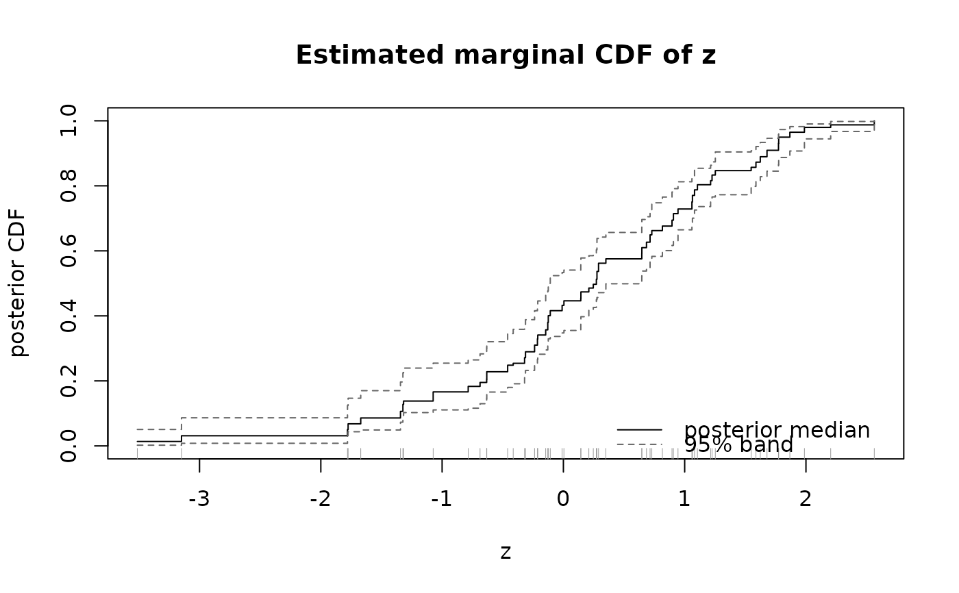
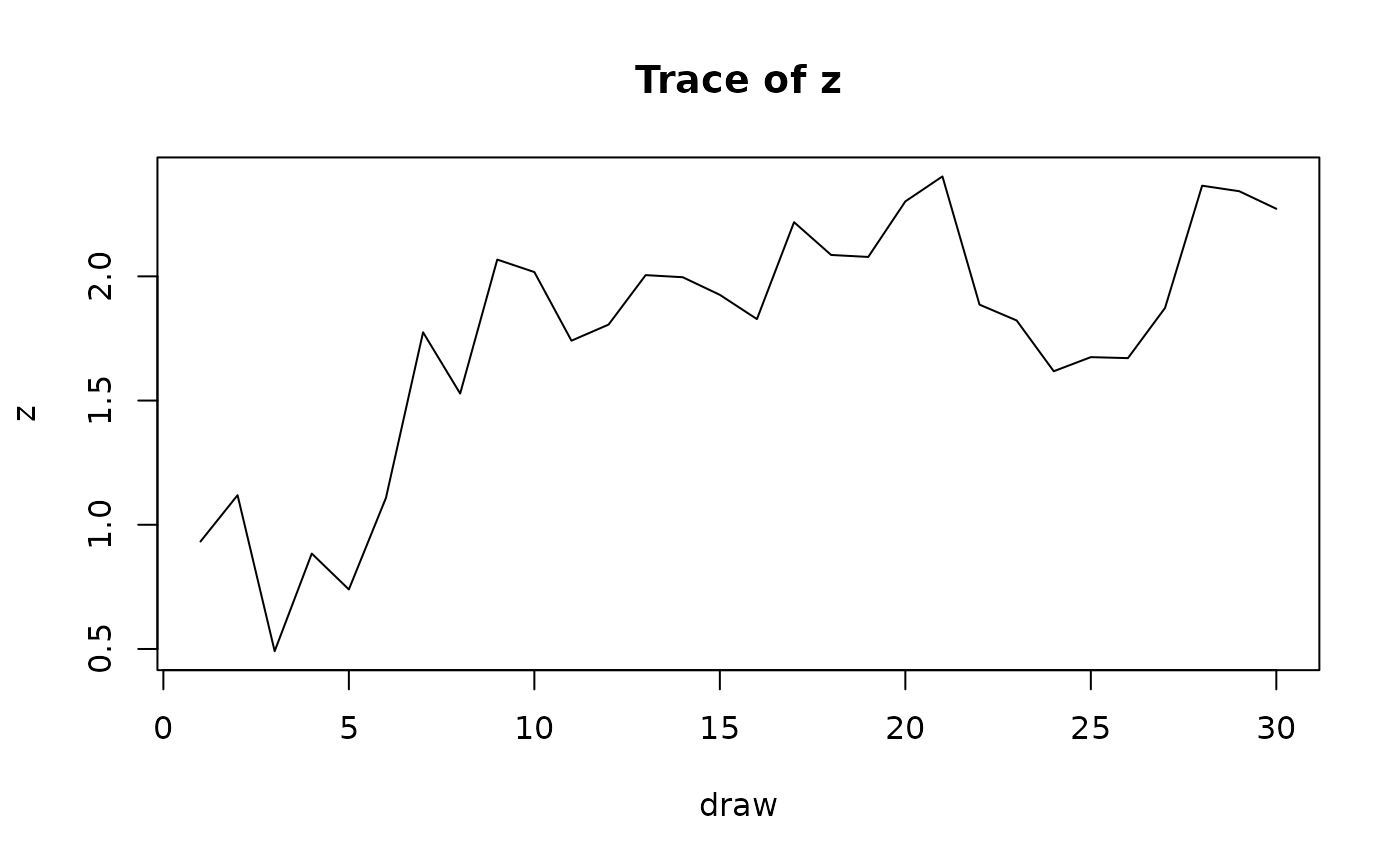
type: One of "trace" (the sampled values against iteration number), "acf" or "pacf" (autocorrelation and partial autocorrelation of the draws), "density" (a kernel density estimate of the posterior with the mean marked), or "cdf" (the posterior of the regressor's marginal CDF, i.e. the cumulative sums of its probability masses, shown as a step function with a pointwise credible band across the draws – an object that has no counterpart in the frequentist estimators, where the CDF is a fixed plug-in with no uncertainty attached). Defaults to "trace".
level: Credible level for the band shown when type = "cdf". Defaults to 0.95.
ask: Whether to prompt between plots when more than one is drawn. Defaults to TRUE on an interactive, multi-plot device and FALSE otherwise.
...: Further arguments passed to the underlying graphics::plot (or stats::acf / stats::pacf) call.

Value

x, invisibly. Called for its side effect of drawing a plot.

References

Haschka, R. E. (2025). Bayesian inference for joint estimation models using copulas to handle endogenous regressors. Oxford Bulletin of Economics and Statistics. doi:10.1111/obes.70023

Examples

set.seed(1)
n <- 60
x <- rnorm(n); z <- x + rnorm(n); y <- 1 + z + x + rnorm(n)
fit <- CopRegBAYES(y ~ z | x, data = data.frame(y, z, x),
                    iterations = 200, burnin = 50, thin = 5, verbose = FALSE)
plot(fit, which = "z", type = "trace")

plot(fit, which = "z", type = "cdf")