8.7 Cluster feasibility

Before applying the clustering algorithm, it is best to assess if the data will yield any meaningful clusters. One popular method is Hopkin’s statistic that tests whether data has uniform distribution. Clustering is only possible when the distribution shows heterogeneous regions. Hopkin’s statistic ranges between 0 and 1. Depending on the way the formula is implemented in the package, clusterability of the data is determined by how close Hopkin’s statistic is to 0 or 1. We will use get_clust_tendency() from factoextra package. According to this function the closer Hopkin’s statistic is to 0, the better is the clusterability in the data.

This function also output a plot showing the clusters. The plot looks at the dissimilarity matrix by computing the distance between points. We ideally want to see blocks of similar color.

set.seed(4569)

cluster_td <- 
  get_clust_tendency(
    cluster_data_pro,
    n = 400, # Pick 400 points randomly
    gradient = list(low = "steelblue",  
                    high = "white")
    )

Print Hopkin’s statistic

cluster_td$hopkins_stat

## [1] 0.03101145

Hopkin’s stat is close to zero, which suggests that data is clusterable. Let’s take a look at Figure 8.1, which also supports that there are blocks of data that can be clustered.

cluster_td$plot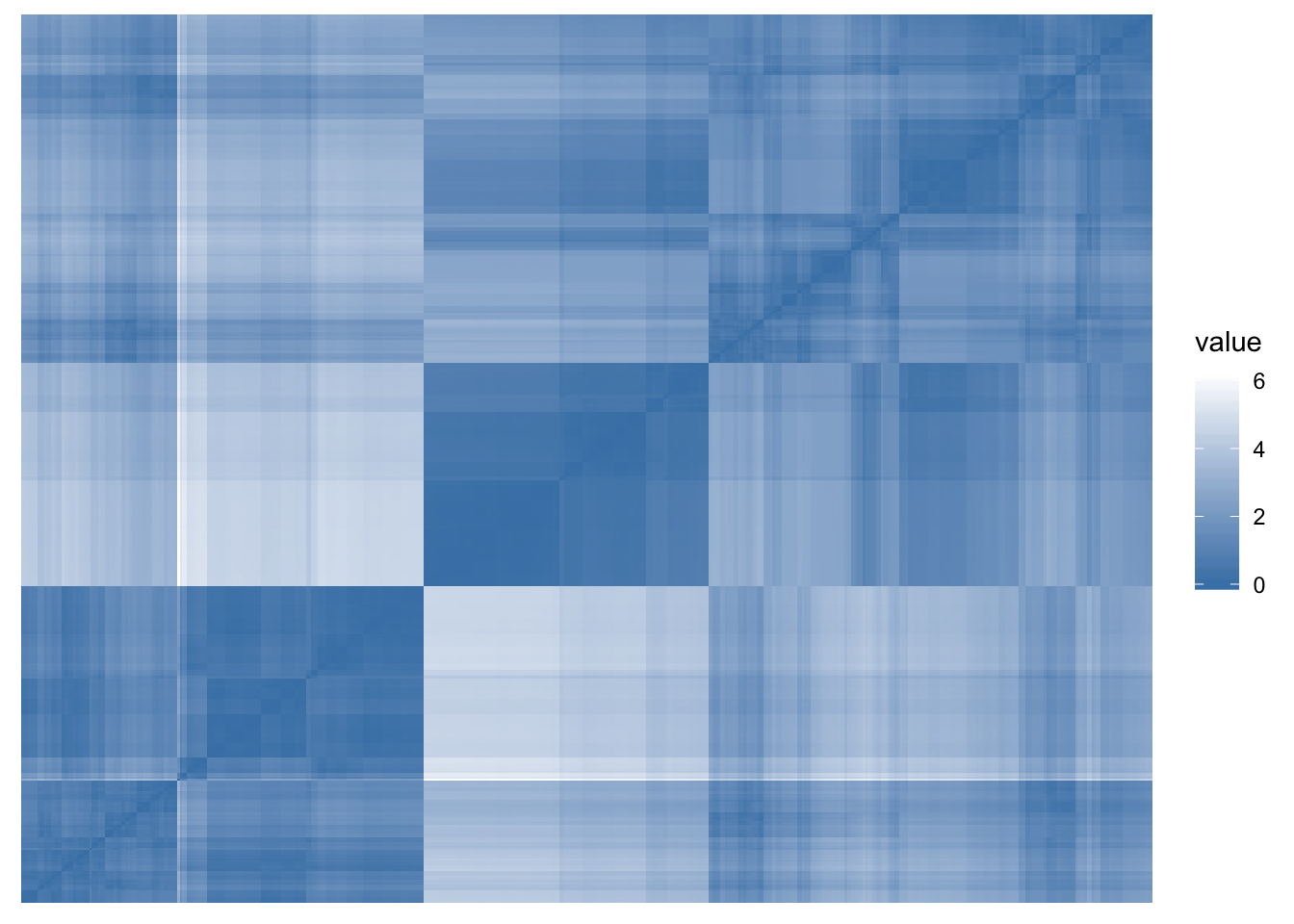

Figure 8.1: Cluster Feasibility Plot