3.10 Support Vector Machines (SVM)
The advantage of using SVM is that although it is a linear model, we can use kernels to model linearly non-separable data. We will use the default radial basis function (RBF) kernel for SVM. An SVM with RBF takes two hyper parameters that we need to tune before estimating SVM. But it takes a long time to tune. Therefore, in this example I won’t actually tune it because I have already done it previously using e1071 package.
We will use e1071 and caret separately to get SVM.
Use the following code to estimate SVM using e1071 package.
3.10.1 Hyperparameters tuning
For SVM with RBF, we need to tune gamma and cost hyperparameters. Whereas cost is generic to SVM with any kernel function, gamma is specific to RBF kernel, which is given as follows:
\[\small K(x_i, x_j) = e^{(-\gamma||x_i-x_j||^2)}\]
where \(\small x_i\) are the sample points and \(\small x_j\) are the support vectors. \(\small \gamma\) controls the extent to which support vectors exert influence on classification of any sample point.18
Higher values of gamma will lead to higher in-sample error (high bias) and lower out-of-sample error (low variance).
cost decides the penalty we want to set for not classifying sample points correctly. Therefore, lower cost will lead to more accommodating behavior leading to higher in-sample error (high bias) and lower out-of-sample error (low variance).
# Use multiple cores on your computer
# Change the number of cores depending on your processer

doParallel::registerDoParallel(cores = 4)

set.seed(1234)
svm.tune <- tune.svm(quality.c ~ .,
                     data = train_wine[, -c(12,15)],
                     gamma = c(0.05, 0.1, 0.5, 1, 2),
                     cost = 10^(0:3))
Print the best gamma and cost
svm.tune$best.parameters## gamma cost
## 19 1 1000We find that gamma = 1 and cost = 1000 give us the best accuracy. You can also print the table for the performance of the entire grid by running the following code. This is not executed for this example.
svm.tune$performances3.10.2 Model estimation
Using the best hyperparameters we can estimate the model. In the next code block I will use the hyperparameters from the first pass. Note that the summary() function for svm() doesn’t provide any model parameters.
model.svm.c <- e1071::svm(quality.c ~ .,
                          data = train_wine[, -c(12, 15)],
                          kernel = "radial",
                          gamma = 1,
                          cost = 1000)
Print the model summary. Note that the summary() function for svm() doesn’t provide any model parameters.
summary(model.svm.c)##
## Call:
## svm(formula = quality.c ~ ., data = train_wine[, -c(12, 15)],
## kernel = "radial", gamma = 1, cost = 1000)
##
##
## Parameters:
## SVM-Type: C-classification
## SVM-Kernel: radial
## cost: 1000
##
## Number of Support Vectors: 4389
##
## ( 1393 1899 751 346 )
##
##
## Number of Classes: 4
##
## Levels:
## q_5 q_6 q_7 q_3489We have 4,389 support vectors. This suggests that the model is memorizing rather than learning as the training data set has only 5,200 observations. This could be because of many factors but th emost critical factor is that the predictor variables do not have much information to predict the wine quality.
3.10.3 Assessing the model performance
caret::confusionMatrix(reference = test_wine$quality.c,
                       predict(model.svm.c,
                               newdata = test_wine[, -c(12, 14, 15)],
                               type = "class"))
## Confusion Matrix and Statistics
##
## Reference
## Prediction q_5 q_6 q_7 q_3489
## q_5 398 13 2 3
## q_6 26 543 13 6
## q_7 0 10 199 2
## q_3489 3 1 1 77
##
## Overall Statistics
##
## Accuracy : 0.9383
## 95% CI : (0.9238, 0.9508)
## No Information Rate : 0.4372
## P-Value [Acc > NIR] : <2e-16
##
## Kappa : 0.9072
##
## Mcnemar's Test P-Value : 0.1005
##
## Statistics by Class:
##
## Class: q_5 Class: q_6 Class: q_7 Class: q_3489
## Sensitivity 0.9321 0.9577 0.9256 0.87500
## Specificity 0.9793 0.9384 0.9889 0.99586
## Pos Pred Value 0.9567 0.9235 0.9431 0.93902
## Neg Pred Value 0.9671 0.9661 0.9853 0.99095
## Prevalence 0.3292 0.4372 0.1658 0.06785
## Detection Rate 0.3069 0.4187 0.1534 0.05937
## Detection Prevalence 0.3207 0.4534 0.1627 0.06322
## Balanced Accuracy 0.9557 0.9480 0.9572 0.93543It looks like SVM classification on the data is far better than MNL! We get the model accuracy up to 67% from a mere 54% for MNL. Recall that the no information rate is only 44% so with SVM we could improve the accuracy by 23%.
3.10.4 SVM with caret
The following code will tune the model but it’s actually not going to run in this tutorial because it will take a lot of time.
ctrl <- caret::trainControl(method = "cv",
                            number = 10)

set.seed(1492)
grid <- expand.grid(sigma = 10^(-1:4),
                    C = 10^(0:4))

model.svm.tune <- train(quality.c ~ .,
                        data = train_wine[ , -c(12, 15)],
                        method = "svmRadial",
                        tuneGrid = grid,
                        trControl = ctrl)
Print the best parameter combination.
model.svm.tune$bestTune## sigma C
## 8 1 100We will use sigma = 1 and cost = 100 and estimate the model. We will then use varImp in caret to get the variable importance. In order to plot variable importance, all the predictor variables have to be non-character. As we have a factor variable, wine, we should create a indicator dummy ourselves.
train_wine$white_wine = ifelse(train_wine$wine == "white", 1, 0)
test_wine$white_wine = ifelse(test_wine$wine == "white", 1, 0)
With the best parameters, estimate the model.
ctrl <- caret::trainControl(method = "cv",
                            number = 10)

grid <- expand.grid(sigma = 1, C = 100)

set.seed(89753)

model.svm.c1 <- train(quality.c ~ .,
                     data = train_wine[,-c(12, 13, 15)],
                     method = "svmRadial",
                     tuneGrid = grid,
trControl = ctrl)print(model.svm.c1)## Support Vector Machines with Radial Basis Function Kernel
##
## 5200 samples
## 12 predictor
## 4 classes: 'q_5', 'q_6', 'q_7', 'q_3489'
##
## No pre-processing
## Resampling: Cross-Validated (10 fold)
## Summary of sample sizes: 4680, 4679, 4680, 4679, 4679, 4681, ...
## Resampling results:
##
## Accuracy Kappa
## 0.6426823 0.4405893
##
## Tuning parameter 'sigma' was held constant at a value of 1
##
## Tuning parameter 'C' was held constant at a value of 100In-sample accuracy of the model is 64%. Next, we will check the number of support vectors. Similar to the SVM fitted using e1071, we get 4,386 support vectors using caret, which underneath uses kernlab package.
model.svm.c1$finalModel## Support Vector Machine object of class "ksvm"
##
## SV type: C-svc (classification)
## parameter : cost C = 100
##
## Gaussian Radial Basis kernel function.
## Hyperparameter : sigma = 1
##
## Number of Support Vectors : 4386
##
## Objective Function Value : -3306.48 -728.0289 -516.7598 -1715.672 -660.8427 -485.7019
## Training error : 0.0001923.10.5 Model performance
We test the SVM performance using test_wine
caret::confusionMatrix(reference = test_wine$quality.c,
                       predict(model.svm.c1,
                               newdata = test_wine[, -c(12, 13, 14, 15)],
                               type = "raw"))
## Confusion Matrix and Statistics
##
## Reference
## Prediction q_5 q_6 q_7 q_3489
## q_5 398 13 2 3
## q_6 26 543 14 6
## q_7 0 10 198 2
## q_3489 3 1 1 77
##
## Overall Statistics
##
## Accuracy : 0.9375
## 95% CI : (0.923, 0.9501)
## No Information Rate : 0.4372
## P-Value [Acc > NIR] : < 2e-16
##
## Kappa : 0.9061
##
## Mcnemar's Test P-Value : 0.09136
##
## Statistics by Class:
##
## Class: q_5 Class: q_6 Class: q_7 Class: q_3489
## Sensitivity 0.9321 0.9577 0.9209 0.87500
## Specificity 0.9793 0.9370 0.9889 0.99586
## Pos Pred Value 0.9567 0.9219 0.9429 0.93902
## Neg Pred Value 0.9671 0.9661 0.9844 0.99095
## Prevalence 0.3292 0.4372 0.1658 0.06785
## Detection Rate 0.3069 0.4187 0.1527 0.05937
## Detection Prevalence 0.3207 0.4541 0.1619 0.06322
## Balanced Accuracy 0.9557 0.9473 0.9549 0.93543At 66.7%, the model accuracy is comparable to the SVM estimated using e1071. Overall, SVM improved the model accuracy significantly over MNL.
3.10.6 Variable importance
Next, let’s plot the variable importance using ggplot2.19
var.imp <- varImp(model.svm.c1,
                  scale = TRUE)

var.imp2 <- var.imp$importance

var.imp2$Chemistry <- rownames(var.imp2)

# Transpose the data
var.imp2 <- reshape2::melt(var.imp2, id = c("Chemistry"))

ggplot(data = var.imp2, aes(x = Chemistry, y = value)) +
   geom_col(aes(fill = variable)) +
   facet_wrap(~variable) +
   scale_fill_manual(values = c("#d08770", "#ebcb8b", "#a3be8c", "#b48ead")) +
   xlab(NULL) +
   ylab("Importance Weight") +
   theme_minimal() +
   theme(axis.text.x = element_text(angle = 60, hjust = 1),
            legend.position = "none")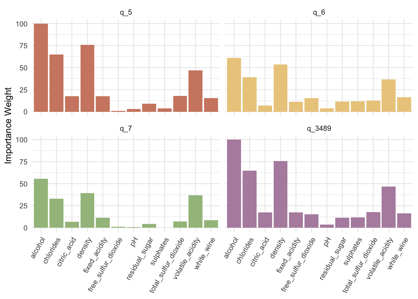
Similar to MNL, we have each predictor with different effectiveness in predicting different classes. Clearly alcohol content looks like the most important predictor for all the classes.
In summary, SVM performs really well compared to MNL. Note that we have been using quality.c as our target variable, which assumes there is no ordering in quality. Thus, even with limited imformation, SVM performed really well.