5.6 Sentiment analysis
We will do some basic sentiment analysis. The objective is to find out the general sentiment in our tweets. The variable of interest here is text, which has all the tweet text. We will use lexicon-based method to identify the sentiment in each tweet first and then we will aggregate them all. For this, we will use get_nrc_sentiment() function from syuzhet package. Note that the execution takes some time so please be patient.
lp_sent <- lp$text %>%
    syuzhet::get_nrc_sentiment()
Take a peek at the data
head(lp_sent) %>%
knitr::kable(caption = "Twitter Sentiment")| anger | anticipation | disgust | fear | joy | sadness | surprise | trust | negative | positive |
|---|---|---|---|---|---|---|---|---|---|
| 0 | 2 | 0 | 0 | 0 | 0 | 0 | 0 | 0 | 1 |
| 0 | 0 | 0 | 0 | 0 | 0 | 0 | 0 | 0 | 0 |
| 0 | 0 | 0 | 0 | 0 | 0 | 0 | 1 | 0 | 0 |
| 0 | 1 | 0 | 0 | 1 | 0 | 1 | 1 | 0 | 2 |
| 0 | 0 | 0 | 1 | 0 | 1 | 0 | 3 | 1 | 2 |
| 0 | 0 | 0 | 0 | 0 | 0 | 0 | 0 | 0 | 0 |
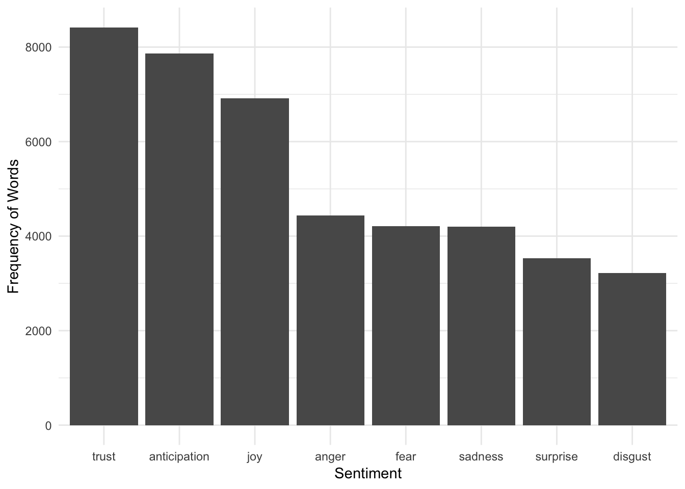
In the above table, the numbers mean the number of words in each tweet that fall into that specific sentiment category. So the first tweet has 2 words indicating anticipation and fifth tweet has 3 words indicating trust. It’s better to aggregate the sentiments and plot them for easy interpretations.
lp_sent %>%
  summarize_all(sum, na.rm = TRUE) %>%
  select(-negative, -positive) %>% # Dropping these helps in plotting
  reshape2::melt() %>%
  ggplot(aes(reorder(variable, -value), value)) +
  geom_col() +
  labs(x = "Sentiment", y = "Frequency of Words") +
  theme_minimal()
## No id variables; using all as measure variables
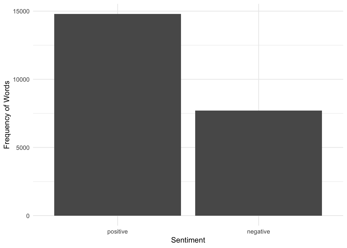
Plot only positive and negative sentiment.
lp_sent %>%
  summarize_all(sum, na.rm = TRUE) %>%
  select(negative, positive) %>%
  reshape2::melt() %>%
  ggplot(aes(reorder(variable, -value), value)) +
  geom_col() +
  labs(x = "Sentiment", y = "Frequency of Words") +
  theme_minimal()
## No id variables; using all as measure variables
Certainly, the tweets have a lot of positive sentiment! But does that matter to make tweets more popular?
5.6.1 Linear regression
In order to find out whether the sentiment can affect the count of favorites, we will do linear regression analysis. We will regress log of favorite_count on the sentiment counts as well as whether the tweets is verified and log of followers_count. As both the counts can be 0, we add 1 to them before taaking the log.
cbind(lp, lp_sent) %>%
  mutate(favorite_count = favorite_count + 1) %>%
  lm(log(favorite_count) ~ anger + anticipation + disgust + fear + joy +
             sadness + surprise + trust + verified + log(followers_count + 1),
           data = .) %>%
  summary()
##
## Call:
## lm(formula = log(favorite_count) ~ anger + anticipation + disgust +
## fear + joy + sadness + surprise + trust + verified + log(followers_count +
## 1), data = .)
##
## Residuals:
## Min 1Q Median 3Q Max
## -2.9398 -0.5172 -0.2173 0.3306 6.6115
##
## Coefficients:
## Estimate Std. Error t value Pr(>|t|)
## (Intercept) -0.496412 0.023189 -21.407 < 2e-16 ***
## anger 0.011007 0.016752 0.657 0.511160
## anticipation -0.008309 0.012225 -0.680 0.496708
## disgust 0.010000 0.018799 0.532 0.594749
## fear 0.020153 0.016476 1.223 0.221276
## joy 0.065785 0.013607 4.835 1.34e-06 ***
## sadness -0.007841 0.016786 -0.467 0.640449
## surprise -0.048582 0.015825 -3.070 0.002144 **
## trust 0.033538 0.009916 3.382 0.000721 ***
## verifiedTRUE 1.029077 0.039416 26.108 < 2e-16 ***
## log(followers_count + 1) 0.169462 0.003829 44.257 < 2e-16 ***
## ---
## Signif. codes: 0 '***' 0.001 '**' 0.01 '*' 0.05 '.' 0.1 ' ' 1
##
## Residual standard error: 0.7896 on 17894 degrees of freedom
## Multiple R-squared: 0.1976, Adjusted R-squared: 0.1971
## F-statistic: 440.5 on 10 and 17894 DF, p-value: < 2.2e-16So, it looks like joyful and trusting tweets are favorited a lot while tweets with surprise are less favorited. Note that I have controlled for the follower count as well as whether the account was verified. Both these variables are highly significant.30
As an exercise, rerun the above regression using
retweet_countas the dependent variable.↩