3.6 Predictor variables
Now that we have new dependent variables, let’s take a look at the predictor variables. As we are doing a predictive analysis (we have no plan to do a statistical inference), let’s understand the distribution and correlations of the variables and explore the need for transformation.
For this we will first get the descriptive statistics and correlations for all the numeric variables. Table 3.1 shows the correlations.
cormat <- round(cor(as.matrix(wine[,-c(13,14,15)])),2)
cormat[upper.tri(cormat)] <- ""
cormat <- as.data.frame(cormat) %>% select(-quality)
colnames(cormat) <- c("V1", "V2", "V3", "V4", "V5",
                      "V6", "V7", "V8", "V9", "V10", "V11")
rownames(cormat) <- paste(c(colnames(cormat), "V12"),
                          ":",
                          rownames(cormat))
print(cormat)| V1 | V2 | V3 | V4 | V5 | V6 | V7 | V8 | V9 | V10 | V11 | |
|---|---|---|---|---|---|---|---|---|---|---|---|
| V1 : fixed_acidity | 1 | ||||||||||
| V2 : volatile_acidity | 0.22 | 1 | |||||||||
| V3 : citric_acid | 0.32 | -0.38 | 1 | ||||||||
| V4 : residual_sugar | -0.11 | -0.2 | 0.14 | 1 | |||||||
| V5 : chlorides | 0.3 | 0.38 | 0.04 | -0.13 | 1 | ||||||
| V6 : free_sulfur_dioxide | -0.28 | -0.35 | 0.13 | 0.4 | -0.2 | 1 | |||||
| V7 : total_sulfur_dioxide | -0.33 | -0.41 | 0.2 | 0.5 | -0.28 | 0.72 | 1 | ||||
| V8 : density | 0.46 | 0.27 | 0.1 | 0.55 | 0.36 | 0.03 | 0.03 | 1 | |||
| V9 : pH | -0.25 | 0.26 | -0.33 | -0.27 | 0.04 | -0.15 | -0.24 | 0.01 | 1 | ||
| V10 : sulphates | 0.3 | 0.23 | 0.06 | -0.19 | 0.4 | -0.19 | -0.28 | 0.26 | 0.19 | 1 | |
| V11 : alcohol | -0.1 | -0.04 | -0.01 | -0.36 | -0.26 | -0.18 | -0.27 | -0.69 | 0.12 | 0 | 1 |
| V12 : quality | -0.08 | -0.27 | 0.09 | -0.04 | -0.2 | 0.06 | -0.04 | -0.31 | 0.02 | 0.04 | 0.44 |
Next we will use ggcorrplot package to create a nice looking correlation plot. This package is available on CRAN
ggcorrplot::ggcorrplot(round(cor(as.matrix(wine[, -c(13,14,15)])), 2),
            p.mat = ggcorrplot::cor_pmat(as.matrix(wine[, -c(13,14,15)])),
            hc.order = TRUE, type = "lower",
            outline.col = "white",
            ggtheme = ggplot2::theme_minimal,
            colors = c("#cf222c", "white", "#3a2d7f")
            )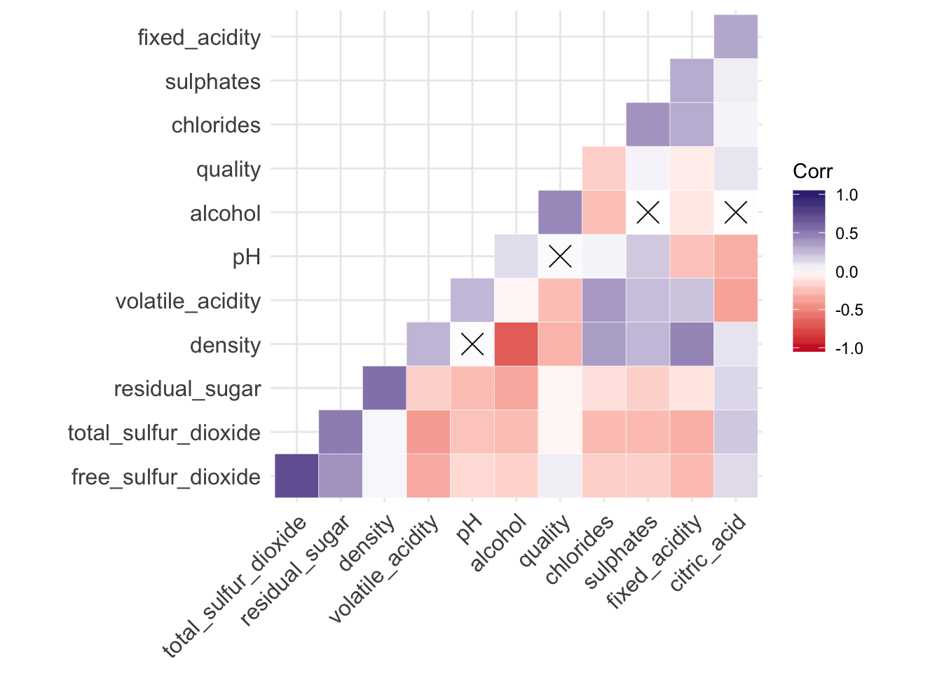
Figure 3.1: Correlation Heatmap
In the above heat map, the crosses indicate non-significant correlations. From the correlations, most variables have their own unique information set. However, it appears that quality is strongly related to only a few variables. This is not great news!12
At this point one can think of transformations to increase the correlations between the variables. However, I am not going to do it as this will make this exercise broader than I want. This is left to the reader as an exercise.↩