5.7 Create a wordcloud

Wordcloud is a popular visualization tool, yet I am not a big fan of it. However, it seems that managers love a wordcloud because they can get the main message in one quick look. We will create a wordcloud using eom_text_wordcloud() function from ggwordcloud package.

Before we can make a wordcloud, there is some preprocessing of the text that is necessary. First of all, we need to tokenize the text so that we have all the words separately identified. Next, we get rid of all the “stop words” such as articles (e.g., the, an), pronouns (e.g., he, she, it), etc. We also need to remove other words that we think may contaminate the wordcloud.³¹

Create a tibble of all the words we want to get rid of. This list needs to be updated depending on what shows up in the wordcloud below.

exclude_words <- tibble(word = c("http", "https", "twitter", "t.co",
                                 "liverpool", "barcelona", "barca"))

We have to first get the words from all the tweets

word_tokens <- lp_geo %>% 
  select(status_id, text) %>% 
  tidytext::unnest_tokens(word, text) %>% 
  anti_join(stop_words) %>% 
  anti_join(exclude_words)

## Joining, by = "word"
## Joining, by = "word"

head(word_tokens)

## # A tibble: 6 x 2
##   status_id           word           
##   <chr>               <chr>          
## 1 1125931671986028544 poznaninmypants
## 2 1125931671986028544 destnd4gr8tnes2
## 3 1125931671986028544 yankeegunner   
## 4 1125931671986028544 gunnerblog     
## 5 1125931671986028544 clivepafc      
## 6 1125931671986028544 vision

The first few words that we see are probably hashtags this user used. We don’t need to pay attention to individual words at this point.

Find the frequency of each word and then rank them in descending order

word_tokens_count <- word_tokens %>% 
  count(word, sort = TRUE)

head(word_tokens_count)

## # A tibble: 6 x 2
##   word       n
##   <chr>  <int>
## 1 league  1692
## 2 final   1647
## 3 win     1599
## 4 game    1358
## 5 team    1335
## 6 0       1330

Make the wordcloud

set.seed(2019)

word_tokens_count %>% 
  top_n(30) %>% 
  ggplot(aes(label = word, size = n, color = word)) +
  scale_size_area(max_size = 10) +
  geom_text_wordcloud() +
  theme_minimal()

## Selecting by n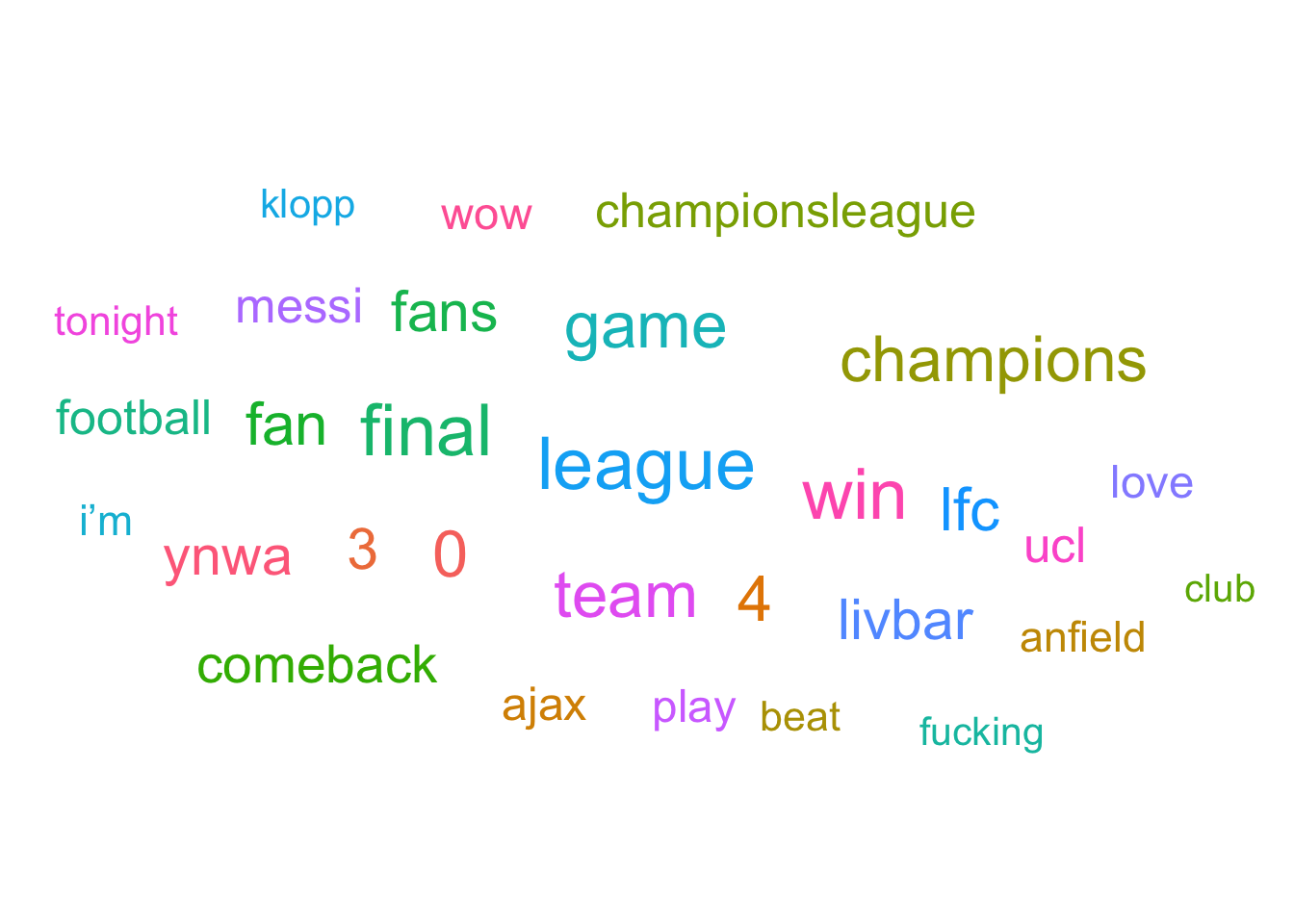

Another way you can create wordcloud quickly is using a custom R function available from STHDA

source('http://www.sthda.com/upload/rquery_wordcloud.r')

Full wordcloud. The default is to plot 200 words.

rquery.wordcloud(x = lp$text, type = "text")

Wordcloud without the excluded words:

rquery.wordcloud(x = lp$text, type = "text",
                 excludeWords = c("http", "https", "twitter", "t.co",
                                 "liverpool", "barcelona", "barca"),
                 max.words = 50)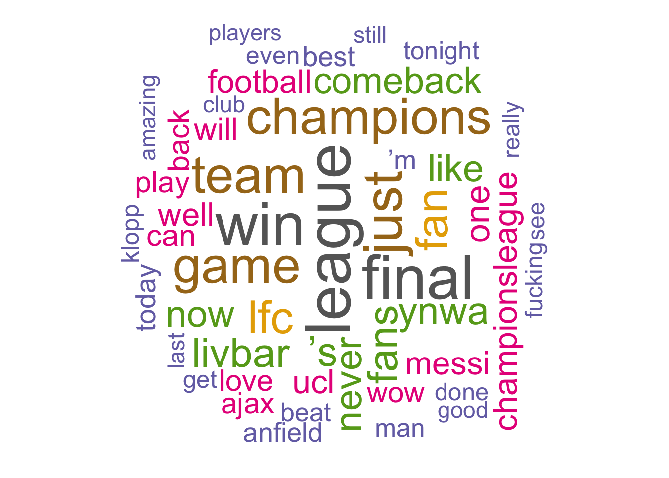

This requires some trial and error.↩