6.6 The moment of truth
Now comes the final stage where we check the correlations between various NSS measures and ACSI. For this I use ggcorplot() function from ggcorplot package. As this is not a major topic for this exercise, I leave the explanation of the code to you as an exercise.
ggcorrplot::ggcorrplot(
  airlines_final %>%
    select(starts_with("nss"), acsi) %>%
    cor() %>%
    round(2),
  p.mat = ggcorrplot::cor_pmat(
    airlines_final %>%
      select(starts_with("nss"), acsi)
    ),
  hc.order = TRUE,
  type = "lower",
  outline.color = "white",
  ggtheme = ggplot2::theme_minimal,
  colors = c("#cf222c", "white", "#3a2d7f")
  )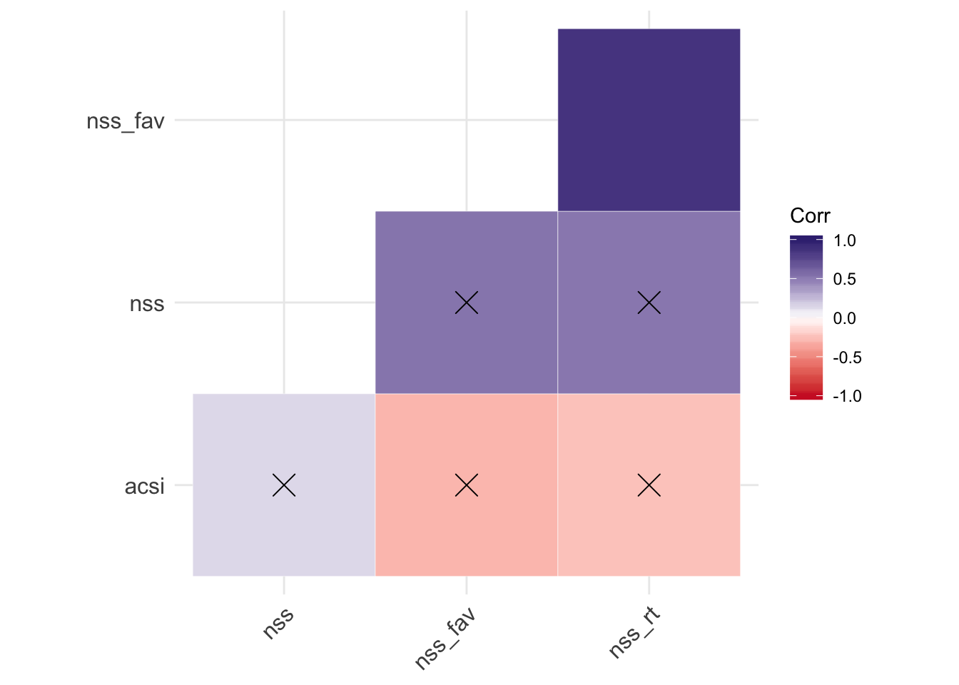
Figure 6.1: Correlation Plot
From Figure 6.1 it looks like ACSI has somewhat negative correlations with each of the NSS metric! This is not good news…for ACSI! :)Furthermore, the crosses on the squares indicate statistical non-significance. However, as I explain below, we will do a better comparison with more direct sentiment metrics.
Table 6.3 shows the correlations in numbers. Indeed, ACSI is marginally negatively correlated with NSS metrics.
| nss | nss_fav | nss_rt | acsi | |
|---|---|---|---|---|
| nss | 1.000 | 0.528 | 0.518 | 0.138 |
| nss_fav | 0.528 | 1.000 | 0.857 | -0.297 |
| nss_rt | 0.518 | 0.857 | 1.000 | -0.251 |
| acsi | 0.138 | -0.297 | -0.251 | 1.000 |