6.7 Correlating with granular sentiments
Thus far we used only positive and negative sentiments. However, we actually have much granular sentiment scores in the data. Let’s check whether these scores do a better job of explaining the pattern in the data.
For this, we will simply use the percentage of words with a specific sentiment in a tweet. For instance, if there were 2 words that were labeled as “joy” by syuzhet out of the 5 words it labeled overall from a tweet, we consider it is 40% (2/5) joy. It’s not the cleanest metric but it will work.
To calculate row percentages, we will use adorn_percentages() function from janitor package. This function has two drawbacks. First, it assumes that the first column is “id” column and it doesn’t take it into account for row calculations. We overcome this problem by adding a column of airlines and then making it the first column using select() function from dplyr. Second, the package returns NaN when the row sums are 0. This is not a drawback in general but our application needs a 0 in place of NaN. We will fix this using is.na() function from base R.
sent_cor <- airlines_sent %>%
    # Add airline names
  mutate(airline = airlines_df$airline) %>%
  select(airline, everything(), -c(positive, negative)) %>%
  janitor::adorn_percentages() %>%
  as.data.frame()

# Replace NaN with 0

sent_cor[is.na(sent_cor)] <- 0

# Finally summarize and add ACSI

sent_cor <- sent_cor %>%
  group_by(airline) %>%
  summarize_if(is.numeric, mean) %>%
  # Add ACSI scores
  mutate(acsi = c(80, 71, 73, 75, 64, 79, 79, 63, 70)) %>%
  select(-airline)
6.7.1 Correlation plot
Figure 6.2 shows the correlation plot.
ggcorrplot::ggcorrplot(
  sent_cor %>%
  cor(method = "pearson") %>%
  round(3),
  p.mat = ggcorrplot::cor_pmat(sent_cor, method = "pearson"),
  hc.order = TRUE,
  type = "lower",
  outline.color = "white",
  ggtheme = ggplot2::theme_minimal,
  colors = c("#cf222c", "white", "#3a2d7f")
  )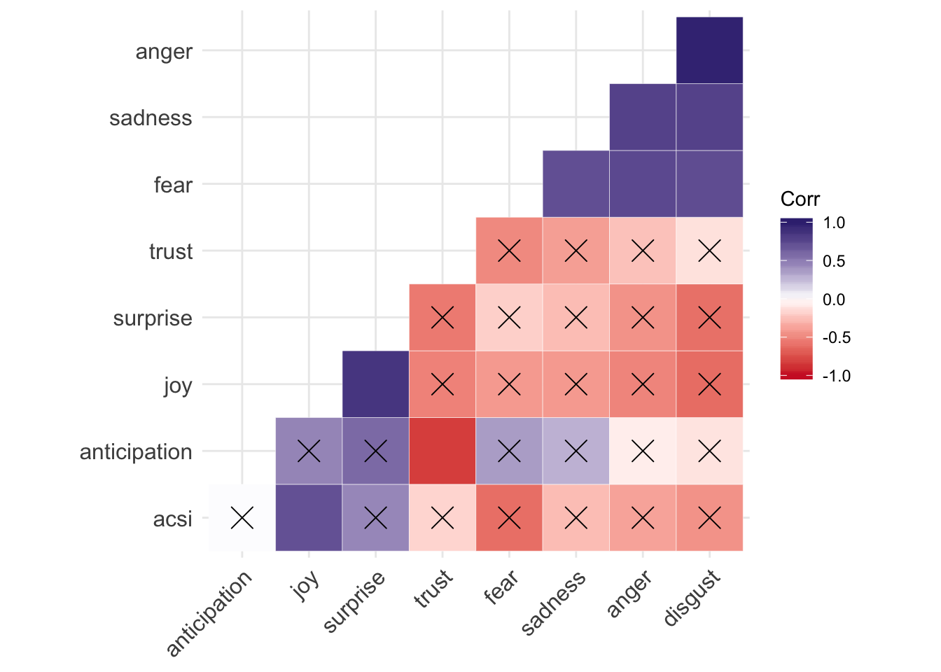
Figure 6.2: Granual Sentiment Correlation Plot
ACSI has positive correlations with joy, surprise, and anticipation. It has negative correlations with the rest. Surprisingly, it has a negative correlation with trust.40 Unfortunately, none of these correlations is statistically significant at 5% level of significance! This is somewhat expected because we have only 9 airlines.
6.7.2 Correlation matrix
Let’s take a look at the correlations as shown in Table 6.4. We will also output the p values this time. For this, we will use rcorr() function from Hmisc package. rcorr() outputs a list with correlations and their p values in separate matrices.
sent_cor %>%
  as.matrix() %>%
  Hmisc::rcorr() %>%
  .$r %>%
round(3)| anger | anticipation | disgust | fear | joy | sadness | surprise | trust | acsi | |
|---|---|---|---|---|---|---|---|---|---|
| anger | 1.000 | -0.073 | 0.966 | 0.738 | -0.513 | 0.783 | -0.449 | -0.250 | -0.377 |
| anticipation | -0.073 | 1.000 | -0.111 | 0.357 | 0.462 | 0.278 | 0.585 | -0.833 | 0.007 |
| disgust | 0.966 | -0.111 | 1.000 | 0.721 | -0.622 | 0.777 | -0.598 | -0.122 | -0.450 |
| fear | 0.738 | 0.357 | 0.721 | 1.000 | -0.418 | 0.714 | -0.193 | -0.490 | -0.611 |
| joy | -0.513 | 0.462 | -0.622 | -0.418 | 1.000 | -0.423 | 0.848 | -0.523 | 0.700 |
| sadness | 0.783 | 0.278 | 0.777 | 0.714 | -0.423 | 1.000 | -0.269 | -0.398 | -0.274 |
| surprise | -0.449 | 0.585 | -0.598 | -0.193 | 0.848 | -0.269 | 1.000 | -0.561 | 0.449 |
| trust | -0.250 | -0.833 | -0.122 | -0.490 | -0.523 | -0.398 | -0.561 | 1.000 | -0.166 |
| acsi | -0.377 | 0.007 | -0.450 | -0.611 | 0.700 | -0.274 | 0.449 | -0.166 | 1.000 |
Table 6.5 shows the p values corresponding to the correlation coefficients. The p value for the correlation coefficient between ACSI and joy is significant at 10% level.
sent_cor %>%
  as.matrix() %>%
  Hmisc::rcorr(type = "pearson") %>%
  .$P %>%
round(3)| anger | anticipation | disgust | fear | joy | sadness | surprise | trust | acsi | |
|---|---|---|---|---|---|---|---|---|---|
| anger | NA | 0.852 | 0.000 | 0.023 | 0.158 | 0.013 | 0.226 | 0.517 | 0.318 |
| anticipation | 0.852 | NA | 0.777 | 0.346 | 0.211 | 0.470 | 0.098 | 0.005 | 0.986 |
| disgust | 0.000 | 0.777 | NA | 0.028 | 0.074 | 0.014 | 0.089 | 0.754 | 0.224 |
| fear | 0.023 | 0.346 | 0.028 | NA | 0.263 | 0.031 | 0.619 | 0.180 | 0.080 |
| joy | 0.158 | 0.211 | 0.074 | 0.263 | NA | 0.257 | 0.004 | 0.148 | 0.036 |
| sadness | 0.013 | 0.470 | 0.014 | 0.031 | 0.257 | NA | 0.484 | 0.289 | 0.476 |
| surprise | 0.226 | 0.098 | 0.089 | 0.619 | 0.004 | 0.484 | NA | 0.116 | 0.225 |
| trust | 0.517 | 0.005 | 0.754 | 0.180 | 0.148 | 0.289 | 0.116 | NA | 0.670 |
| acsi | 0.318 | 0.986 | 0.224 | 0.080 | 0.036 | 0.476 | 0.225 | 0.670 | NA |
Any speculations for this result?↩