4.3 Building the predictive model
We will use random forest for building the predictive model. First define the training controls. The only meaningful hyper parameter that makes substantial difference in accuracy is mtry which is the number of variables to use for building each tree in the random forest. You can tune this hyper parameter by using grid search.
trControl <- trainControl(method = "cv", #crossvalidation
                          number = 10,   # 10 folds
                          search = "grid",
                          classProbs = TRUE  #computes class probabilities
                          )

tuneGrid_large <- expand.grid(mtry = c(1:(ncol(dt4) - 2)))
Now train the model. The code in the next block is for demonstration purposes and I advice you not to run it during the class. This is because it will take several minutes if not hours to execute.
We derive the model by using train() function form caret. We first specify the formula, which in our case is CarInsurance as a function of all the variable sin the model. Next, we specify the data set to be used. caret has numerous machine learning and statistical methods (258 in all). For random forest, we will use rf method. With this method, under the hood, caret is using randomForest package. But note that other alternatives for random forest such as ranger are available as well.21
For classification, we will use “Accuracy” as the metric to maximize. Then we provide the tuning grid and training control objects, and finally select the number of trees.22
Warning: This will take several minutes or even hours to run!
set.seed(9933)

modelRF_large <- train(CarInsurance ~ . ,
                 data = dt4_train,
                 method = "rf",
                 metric = "Accuracy",
                 tuneGrid = tuneGrid_large,
                 trControl = trControl,
                 ntree = 1000)
Now print the model to take a look at the accuracies.
print(modelRF_large)## Random Forest
##
## 3201 samples
## 46 predictor
## 2 classes: 'No', 'Yes'
##
## No pre-processing
## Resampling: Cross-Validated (10 fold)
## Summary of sample sizes: 2882, 2880, 2880, 2881, 2881, 2881, ...
## Resampling results across tuning parameters:
##
## mtry Accuracy Kappa
## 1 0.6660384 0.2024168
## 2 0.7553787 0.4543552
## 3 0.8237960 0.6271341
## 4 0.8384777 0.6632234
## 5 0.8416154 0.6720805
## 6 0.8403644 0.6693719
## 7 0.8441106 0.6775140
## 8 0.8419221 0.6734917
## 9 0.8419211 0.6739009
## 10 0.8419230 0.6739344
## 11 0.8419221 0.6738316
## 12 0.8434836 0.6774717
## 13 0.8387951 0.6673813
## 14 0.8409777 0.6717585
## 15 0.8425412 0.6750726
## 16 0.8406633 0.6718024
## 17 0.8415969 0.6734528
## 18 0.8415998 0.6731690
## 19 0.8453489 0.6815814
## 20 0.8409767 0.6721318
## 21 0.8406662 0.6714256
## 22 0.8431594 0.6767590
## 23 0.8406623 0.6713721
## 24 0.8415978 0.6734469
## 25 0.8431604 0.6770513
## 26 0.8397297 0.6698172
## 27 0.8384738 0.6671387
## 28 0.8381691 0.6663353
## 29 0.8390988 0.6685000
## 30 0.8400353 0.6704002
## 31 0.8387863 0.6678400
## 32 0.8403469 0.6711783
## 33 0.8378488 0.6660378
## 34 0.8381642 0.6662424
## 35 0.8381603 0.6664330
## 36 0.8406643 0.6717384
## 37 0.8419133 0.6744978
## 38 0.8400324 0.6705347
## 39 0.8381603 0.6666285
## 40 0.8381623 0.6666150
## 41 0.8403478 0.6707452
## 42 0.8400314 0.6705115
## 43 0.8394084 0.6692103
## 44 0.8390930 0.6687031
## 45 0.8381584 0.6666179
##
## Accuracy was used to select the optimal model using the largest value.
## The final value used for the model was mtry = 19.We can also make a plot for an easy comparison.
plot(modelRF_large)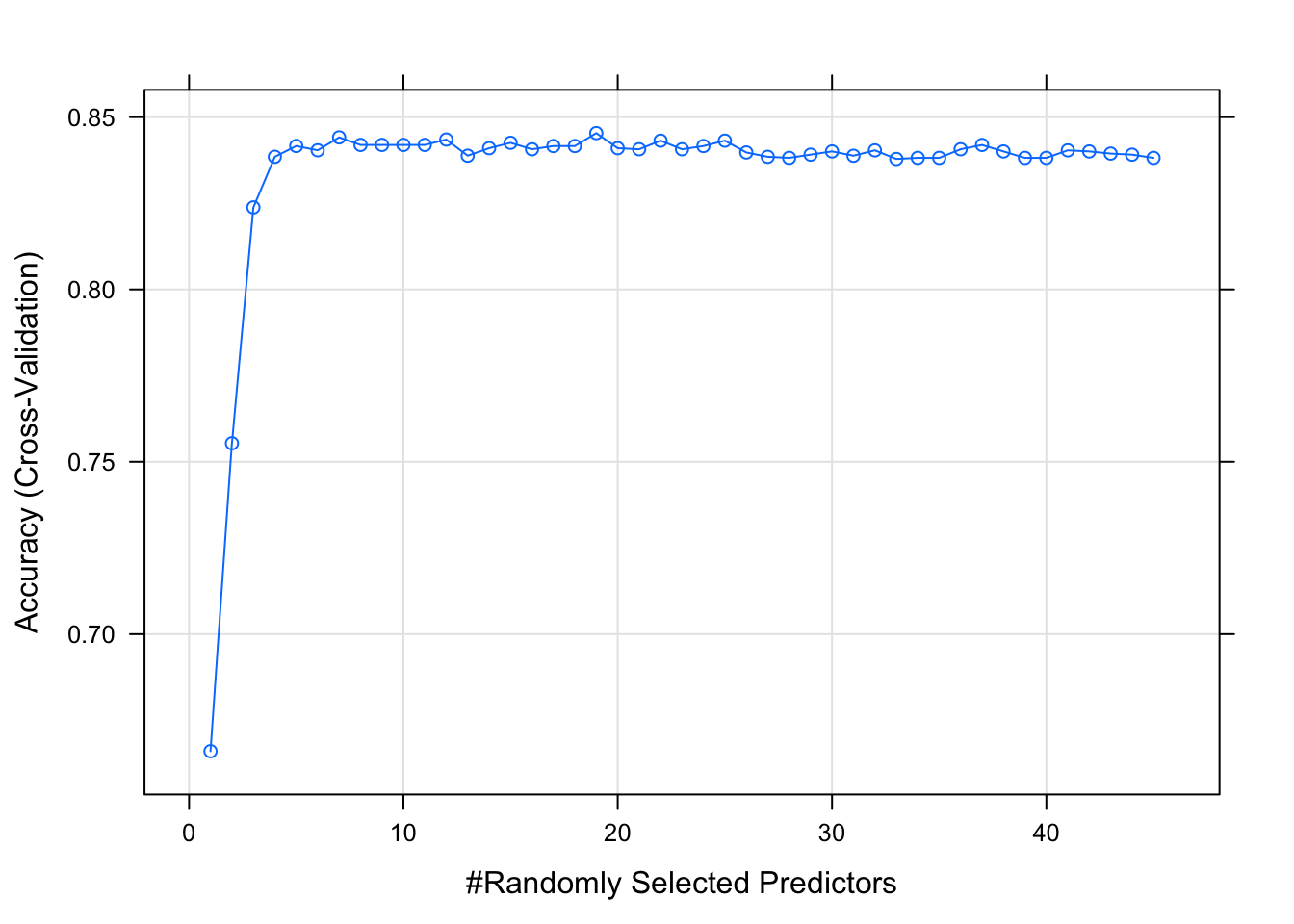
We are getting the highest accuracy when mtry = 19 so I am going to set mtry to 19 for this example. We will execute the code below in the class. However, if you are curious, you could use mtry = 7 as well given that there is a minor difference between the two accuracies. Furthermore, a smaller number of trees is preferred over a larger number because it is likely to perform better out of sample.
4.3.1 Random forest with fixed mtry
Run this code in the class instead of the grid search above.
trControl <- trainControl(method = "cv",
                          number = 10,
                          search = "grid",
                          classProbs = TRUE)

tuneGrid <- expand.grid(mtry = 19)
Next, train the model using the above training controls.
set.seed(9999)

modelRF <- train(CarInsurance ~ . ,
                 data = dt4_train,
                 method = "rf",
                 metric = "Accuracy",
                 tuneGrid = tuneGrid,
                 trControl = trControl,
ntree = 1000)print(modelRF)## Random Forest
##
## 3201 samples
## 46 predictor
## 2 classes: 'No', 'Yes'
##
## No pre-processing
## Resampling: Cross-Validated (10 fold)
## Summary of sample sizes: 2880, 2881, 2881, 2881, 2881, 2880, ...
## Resampling results:
##
## Accuracy Kappa
## 0.8422473 0.6749728
##
## Tuning parameter 'mtry' was held constant at a value of 19Our model has a decent resampling accuracy of 84.2%. Kappa is 0.67, which is also fairly acceptable.23
varImp(modelRF, scale = TRUE)## rf variable importance
##
## only 20 most important variables shown (out of 46)
##
## Overall
## CallDuration 100.000
## Age 16.384
## Outcome3 15.770
## Balance 13.517
## CallEndSec 10.594
## LastContactDay 10.296
## CallEndMin 9.574
## CallStartSec 9.527
## CallStartMin 9.335
## DaysPassed 8.947
## CommunicationNot.Available 8.469
## HHInsurance 8.132
## CallEndHour 5.118
## NoOfContacts 4.962
## CallStartHour 4.742
## PrevAttempts 3.553
## LastContactMonth.mar 3.524
## LastContactMonth.aug 2.892
## CarLoan 2.026
## LastContactMonth.jun 2.009Variance importance suggests that CallDuration is the single-most important variable! Let’s talk more about this below.
confusionMatrix(predict(modelRF, select(dt4_test, -CarInsurance)),
                reference = dt4_test$CarInsurance,
                positive = "Yes")
## Confusion Matrix and Statistics
##
## Reference
## Prediction No Yes
## No 467 7
## Yes 12 313
##
## Accuracy : 0.9762
## 95% CI : (0.9631, 0.9856)
## No Information Rate : 0.5995
## P-Value [Acc > NIR] : <2e-16
##
## Kappa : 0.9506
##
## Mcnemar's Test P-Value : 0.3588
##
## Sensitivity : 0.9781
## Specificity : 0.9749
## Pos Pred Value : 0.9631
## Neg Pred Value : 0.9852
## Prevalence : 0.4005
## Detection Rate : 0.3917
## Detection Prevalence : 0.4068
## Balanced Accuracy : 0.9765
##
## 'Positive' Class : Yes
## The confusion matrix suggests that our model performs well outside the sample as well. However, the variable importance calculated above suggests that CallDuration may have a spurious relationship between the likelihood to buy insurance. This is because when a person is interested in buying the insurance, he/she will spend more time on the call.
For a purely predictive task, this is not a concern. If, for example, given all the information in the data set, we want to predict whether a person bought insurance or not, we will do well with the model we built. However, consider this problem from a marketing manager’s perspective. The manager wants to know whether it makes sense to even make a call to a customer. Because the real cost here is the cost of contacting a prospective buyer. So in order to reduce the cost of contacting them, they would like to build a model based on the information that does not include calls.
So, CallDuration might be a good metric for predicting insurance purchase but it is not a good metric for prescribing who to call. This is because, 1) the call has not happened yet and 2) one can’t simply increase the call length and expect the prospect to buy insurance. If call length is the metric to optimize, salespeople will likely game the system and talk nonsense on the phone just to extend the call.
How about you trying out other random forest methods? Check out https://topepo.github.io/caret/train-models-by-tag.html#Random_Forest↩
Note that
caretdoes not treat the number of trees as a hyper parameter. Therefore, you can’t use it in the tuning grid. If, however, you are really interested in tweaking the number of trees, you should use a for loop.↩In practice Kappa > 0.75 suggests very good model accuracy.↩