9.6 Evaluate recommender performance

Now we are all set to build and test various recommenders. recommenderlab gives us several options. We will test all of them. These are specified using method argument and the possible values are: IBCF, UBCF, POPULAR, RANDOM, SVD and SVDF. RANDOM just presents random items to users and works as a benchmark for model comparisons.

The model evaluation in this case will be done using RMSE and similar metrics. Lower values suggest better model performance.

9.6.1 IBCF

ibcf <- 
  train_movies %>%
  Recommender(method = "IBCF") 

ibcf_eval <- ibcf %>% 
  predict(known_movies, type = "ratings") %>% 
  calcPredictionAccuracy(unknown_movies)

Print the model stats.

print(ibcf_eval)

##     RMSE      MSE      MAE 
## 1.526054 2.328841 1.159514

9.6.2 UBCF

ubcf <- 
  train_movies %>%
  Recommender(method = "UBCF")

ubcf_eval <- ubcf %>% 
  predict(known_movies, type = "ratings") %>% 
  calcPredictionAccuracy(unknown_movies)

Print the model stats.

print(ubcf_eval)

##      RMSE       MSE       MAE 
## 1.0304528 1.0618330 0.8246746

9.6.3 Popular

pop <- 
  train_movies %>%
  Recommender(method = "POPULAR")

pop_eval <- pop %>% 
  predict(known_movies, type = "ratings") %>% 
  calcPredictionAccuracy(unknown_movies)

Print the model stats.

print(pop_eval)

##      RMSE       MSE       MAE 
## 0.9626323 0.9266609 0.7606155

9.6.4 Random

random <- 
  train_movies %>%
  Recommender(method = "RANDOM")

random_eval <- random %>% 
  predict(known_movies, type = "ratings") %>% 
  calcPredictionAccuracy(unknown_movies)

Print the model stats.

print(random_eval)

##     RMSE      MSE      MAE 
## 1.382583 1.911535 1.092926

9.6.5 SVD

svd <- 
  train_movies %>%
  Recommender(method = "SVD")

svd_eval <- svd %>% 
  predict(known_movies, type = "ratings") %>% 
  calcPredictionAccuracy(unknown_movies)

Print the model stats.

print(svd_eval)

##      RMSE       MSE       MAE 
## 1.0361175 1.0735394 0.8315897

9.6.6 SVDF

This might take some time depending on your processor.

svdf <- 
  train_movies %>%
  Recommender(method = "SVDF")


svdf_eval <- svdf %>% 
  predict(known_movies, type = "ratings") %>% 
  calcPredictionAccuracy(unknown_movies)

Print the model stats.

print(svdf_eval)

##      RMSE       MSE       MAE 
## 0.9396889 0.8830153 0.7413634

We can now plot the RMSE of all the recommenders we built.

rbind(ibcf_eval, ubcf_eval, pop_eval, 
      random_eval, svd_eval, svdf_eval) %>% 
  as.data.frame() %>% 
  tibble::rownames_to_column(var = "method") %>% 
  ggplot(aes(x = method, y = RMSE)) +
  geom_col() +
  theme_minimal()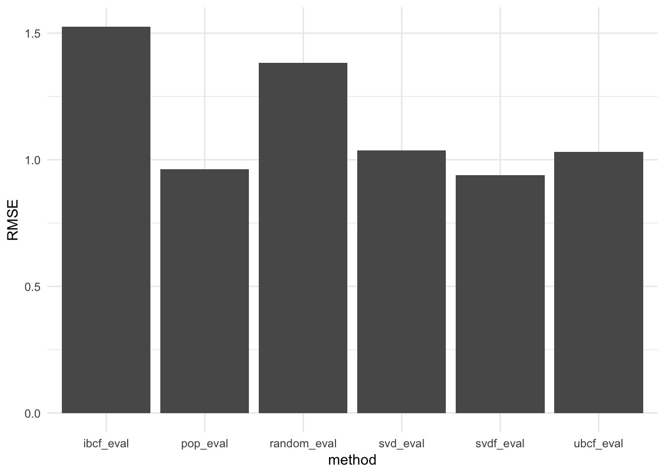

Figure 9.6: Recommender Performance

Figure 9.6 shows the performance of each recommender algorithm. In our case, popular method has done well. This suggests that recommending people the most popular movies is a good option in this data. This is not surprising as Netflix often shows us the popular movies or TV shows. Figure 9.7 shows such recommendations from Netflix.

Figure 9.7: Netflix Popular