5.5 Mapping tweets
As the data obtained is from the US, we should be able to make a map of these tweets very easily. Most people on Twitter do not disclose their location. But as we have a lot of tweets, we will find some of them with their location public. Twitter returned geo_coords variable, which has the latitude and longitude. We will use a handy function from rtweet to extract those.
lp_geo <- lat_lng(lp)Now, we have two new variables lng and lat in the data set.
Next, we create a base map object for 48 states. For this we need to obtain the shape files from the US Census Bureau. Download them from here: https://www.census.gov/geo/maps-data/data/cbf/cbf_state.html and save on your computer.
usa_48 <- sf::st_read(here::here("cb_2017_us_state_20m.shp")) %>%
  filter(!(NAME %in% c("Alaska",
                       "District of Columbia",
                       "Hawaii",
                       "Puerto Rico")))
Plot these using ggplot
ggplot(data = usa_48) +
  geom_sf() +
  theme_minimal()
Now, we will overlay the Twitter data on top of the US map. For this, we will have to convert it into an sf object.
lp_geo_sf <- st_as_sf(filter(lp_geo, !is.na(lat)),
                         coords = c("lng", "lat"))
st_crs(lp_geo_sf) <- 4326   # set the coordinate reference system
Now we are ready to make the plot!
ggplot() +
  geom_sf(data = usa_48, fill = "#2b2b2b") +
  geom_sf(data = lp_geo_sf,
          shape = 16,
          alpha = 0.5,
          color = "#1da1f2") +
  theme_minimal() +
  theme(axis.text.x = element_blank(),
        axis.text.y = element_blank(),
        panel.grid.major = element_blank())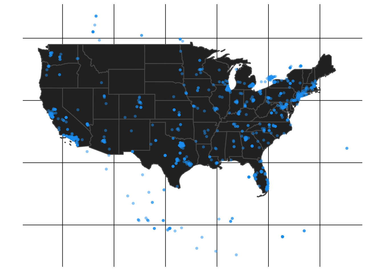
You may try to find some pattern here, but in my experience, Twitter activity is pretty much correlated with the population.