10.9 Random Forest
In order to fit Random Forest, we first specify the control parameters for training. We will use 10-fold cross-validation with 80-20 train and test split. Furthermore, we perform grid search on 18 values of mtry.56
trControl <- trainControl(method = "cv",
                          number = 10,
                          p = 0.8)

tuneGrid <- expand.grid(mtry = 1:18)
Train the model. It will take several hours so I suggest you use tuneGrid = expand.grid(mtry = 1) in the following code.
set.seed(9403)
model_rf <- train(rating ~ . ,
                  data = theta_rating,
                  method = "rf",
                  ntree = 1000,
                  trControl = trControl,
                  tuneGrid = tuneGrid # Use expand.grid(mtry = 1) in the class
                  )
Figure 10.1 shows the model accuracy as a function of mtry. The highest accuracy is obtained when mtry = 1.
model_rf$results %>%
  ggplot(aes(mtry, Accuracy)) +
  geom_line() +
  theme_minimal()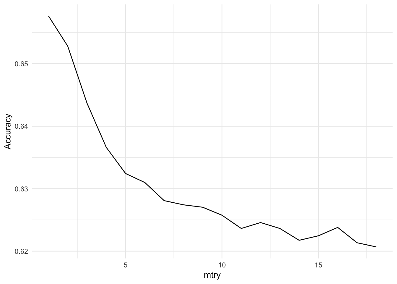
Figure 10.1: Random Forest Tuning
model_rf$bestTune## mtry
## 1 110.9.1 Model performance
Note that we did not split the data into train and test set. As such we will assess model performance on the entire training set. We first get the predicted values of rating based on our model.
rf_predict <- predict(model_rf, theta_rating)Next, we create a confusion matrix using predicted and observed ratings.
confusionMatrix(rf_predict,
                reference = theta_rating$rating)
## Confusion Matrix and Statistics
##
## Reference
## Prediction 1 2 3 4 5
## 1 91 0 0 0 0
## 2 0 81 0 0 0
## 3 0 0 226 0 0
## 4 11 8 21 1314 6
## 5 176 190 676 3377 11784
##
## Overall Statistics
##
## Accuracy : 0.7514
## 95% CI : (0.745, 0.7577)
## No Information Rate : 0.6564
## P-Value [Acc > NIR] : < 2.2e-16
##
## Kappa : 0.3581
##
## Mcnemar's Test P-Value : NA
##
## Statistics by Class:
##
## Class: 1 Class: 2 Class: 3 Class: 4 Class: 5
## Sensitivity 0.327338 0.29032 0.24485 0.28011 0.9995
## Specificity 1.000000 1.00000 1.00000 0.99653 0.2839
## Pos Pred Value 1.000000 1.00000 1.00000 0.96618 0.7273
## Neg Pred Value 0.989536 0.98893 0.96070 0.79658 0.9966
## Prevalence 0.015478 0.01553 0.05139 0.26118 0.6564
## Detection Rate 0.005067 0.00451 0.01258 0.07316 0.6561
## Detection Prevalence 0.005067 0.00451 0.01258 0.07572 0.9021
## Balanced Accuracy 0.663669 0.64516 0.62243 0.63832 0.6417The classification accuracy of Random Forest model is 75%, which is only marginally better than the no information rate of 66%. The no information rate is the relative frequency of “5” rating. In other words, if we predicted that every review has a 5 rating, we will be correct 66% of times.
10.9.2 Variable importance
Finally, it is time to find out the most important topics. The topics that make the most impact on ratings will be considered important. Table 10.1 shows the variable importance. Topics 2, 8, and 10 are the top 3 important topics.
varImp(model_rf, scale = TRUE)| Topics | Overall |
|---|---|
| topic2 | 100.00000 |
| topic8 | 74.32113 |
| topic10 | 40.63719 |
| topic6 | 24.17243 |
| topic17 | 19.08622 |
| topic14 | 15.69933 |
| topic4 | 14.32005 |
| topic5 | 12.87782 |
| topic20 | 12.63768 |
| topic7 | 12.40210 |
In section 10.6 we printed the top 10 words associated with each topic. Let’s print them only for Topics 2, 8, and 10 to get a sense of what these topics are.
terms(lda_model, 10)[, c(2, 8, 10)]## Topic 2 Topic 8 Topic 10
## [1,] "googl" "turn" "charg"
## [2,] "store" "issu" "connect"
## [3,] "android" "star" "wifi"
## [4,] "instal" "reason" "problem"
## [5,] "limit" "bit" "charger"
## [6,] "appl" "review" "issu"
## [7,] "expect" "figur" "plug"
## [8,] "download" "problem" "unit"
## [9,] "load" "button" "power"
## [10,] "function" "open" "replac"It looks like these 3 topics are about complaints pertaining to the Amazon electronics. Topic 2 is about comparison with Google App Store installations, download etc. Topic 8 seems less about the product and more about the review system. Finally, Topic 10 is about WiFi connectivity and charger issues.
Given the distribution of ratings in the data, where 66% of the reviews have 5 rating, it seems logical that the topics related to complaints are helping the model differentiate between the good and bad ratings. This is because reviews with 5 ratings have various topics but none of them with complaints.
I estimated several RFs on various LDAs for this example and I ended up with
mtry = 1as the best hyperparameter in all the cases.↩